|
Go back to main teaching page
|
Theory of series resonance in an LCR circuit
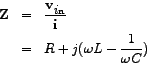
In alternating current (a.c.) theory, all voltages, currents and impedances may be treated as complex quantities. In the series LCR circuit, therefore, the a.c. source (input) voltage
 and the a.c current and the a.c current  are complex and related as follows are complex and related as follows
The corresponding impedance is also complex and is given by
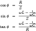
The magnitude of the impedance is
We can then express  in terms of its magnitude as follows in terms of its magnitude as follows
 being the phase angle. From the above equations, we have, being the phase angle. From the above equations, we have,
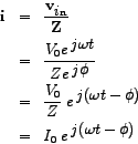
If we express the time-dependent complex source-voltage
as
 , then , then
 and and  being the magnitude of the source-voltage and current respectively. being the magnitude of the source-voltage and current respectively.
Thus we see that the current lags the source-voltage (or alternatively the source-voltage leads the current) by an angle .
Now, if
 or alternatively or alternatively
 , then would be +ve and the current would indeed lag the source-voltage. , then would be +ve and the current would indeed lag the source-voltage.
On the other hand, if
 or alternatively or alternatively
 , then would be -ve and the current would then lead the source-voltage. , then would be -ve and the current would then lead the source-voltage.
Most importantly, if
 or alternatively or alternatively
 , then would be zero and the current and the source-voltage would be `in-phase'. Then , then would be zero and the current and the source-voltage would be `in-phase'. Then  turns out to be equal to turns out to be equal to  and the circuit effectively becomes resistive. Moreover, this value of happens to be the minimum, since is expressed as the square-root of the sum of two squares as shown above. The corresponding magnitude of current, and the circuit effectively becomes resistive. Moreover, this value of happens to be the minimum, since is expressed as the square-root of the sum of two squares as shown above. The corresponding magnitude of current,  , becomes maximum, equalling , becomes maximum, equalling
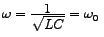
 , and we have Resonance'. The corresponding linear frequncy, viz., , and we have Resonance'. The corresponding linear frequncy, viz.,
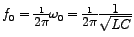 is called the resonant-frequency. is called the resonant-frequency.
In order to graphically follow the time-evolution of the voltages and currents, one needs to plot the waveform profiles. The waveforms are obtained by considering any of the two real parts, viz., the sine or cosine part of the corresponding complex number. For example, since the source-voltage can be written as
the expression for the corresponding waveform may be taken to be
 . Similarly, the current waveform may be expressed as . Similarly, the current waveform may be expressed as
 . .
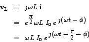
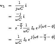
Let us now examine the voltages across the circuit components, ,  and and  . The voltage across is given by . The voltage across is given by
The voltage across is given by
The voltage across is given by
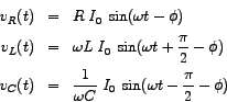
The corresponding real voltages are given by
From the above equations it is clear that the  is `in-phase' with the current, is `in-phase' with the current,  leads the current as also by leads the current as also by
 radians or radians or  , and, , and,  lags the current as also by
radians or . , therefore, leads by lags the current as also by
radians or . , therefore, leads by
 radians or radians or  or in other words and are `out-of-phase'. or in other words and are `out-of-phase'.
It is interesting to note the phase-relationships among the different voltages. At the resonant-frequency, the waveform for would have the maximum amplitude. This is expected, as at resonance, the current in the circuit, , is maximum. Interestingly, at this frequency, and are of the same amplitude, viz.,
 . Since, they are also `out-of-phase', they mutually cancel each other leaving only which then equals the source-voltage . Since, they are also `out-of-phase', they mutually cancel each other leaving only which then equals the source-voltage  . .
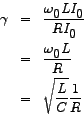
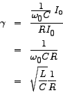
The ratio of the amplitude of the voltage across or (which are equal) at resonance to the amplitude of the source-voltage at resonance is called the voltage-magnification  . The name suggests that the value of the ratio may be much greater than 1 and that is indeed the case. . The name suggests that the value of the ratio may be much greater than 1 and that is indeed the case.
Alternatively
One may draw the phase-versus-frequency plots pertaining to the phase angle , the phase angle for (which is  ), the phase angle for (which is ), the phase angle for (which is
 ) and the phase angle for (which is ) and the phase angle for (which is
 ). ).
From the definition of above and the phase-angle versus frequency plots, we may observe that when the linear-frequency of the source,  , is equal to zero, , is equal to zero,
 . When is equal to the resonant-frequency . When is equal to the resonant-frequency  , ,  . And when is equal to . And when is equal to  , ,
 . .
We may also observe, that as long as
 , or alternatively, , or alternatively,
 , is negative. On the other hand, if , is negative. On the other hand, if
 , or alternatively, , or alternatively,
 , is positive. , is positive.
Besides, at all frequencies, the phase angle for is plus the phase-angle for while the phase angle for is less than the phase-angle for , just as prescribed by theory.
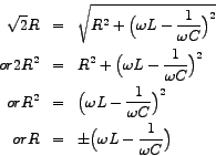
Earlier, we talked of resonance at
 , when the amplitude of the current, viz., , and therefore the amplitude of , becomes maximum. Strictly speaking, we should refer to this resonance as current-resonance. We also have voltage-resonance at two other frequencies, , when the amplitude of the current, viz., , and therefore the amplitude of , becomes maximum. Strictly speaking, we should refer to this resonance as current-resonance. We also have voltage-resonance at two other frequencies,
 and and
 , at which the respective amplitudes of and become maximum. These frequencies can be found by taking the derivatives of the respective amplitudes with respect to the frequency and equating them to zero. They turn out to be: , at which the respective amplitudes of and become maximum. These frequencies can be found by taking the derivatives of the respective amplitudes with respect to the frequency and equating them to zero. They turn out to be:
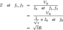
We may also draw the current resonance curve and voltage resonance curves (for
and ). These resonance curves are the response of the respective amplitudes with frequency of the source. It is interesting to observe that
lies to the left of  and
lies to the right of , in agreement with their formulae. We may also plot the magnitude of impedance, , as a function of the frequency. As expected, is minimum and is maximum at the current-resonance frequency, . and
lies to the right of , in agreement with their formulae. We may also plot the magnitude of impedance, , as a function of the frequency. As expected, is minimum and is maximum at the current-resonance frequency, .
If we follow the current-resonance curve, there are two frequencies,  and and  ( (
 ), symmetrically placed on either side of , for which the current-amplitude equals ), symmetrically placed on either side of , for which the current-amplitude equals
 times the maximum value of the current-amplitude . The corresponding power at these two frequencies is therefore half of the power at . and are therefore called 'half-power frequencies'. times the maximum value of the current-amplitude . The corresponding power at these two frequencies is therefore half of the power at . and are therefore called 'half-power frequencies'.
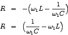
 is called the bandwidth ( is called the bandwidth ( ) of the circuit. An expression for the bandwidth can be obtained as follows: ) of the circuit. An expression for the bandwidth can be obtained as follows:
We also have,
Equating the last two equations, we have,
The  sign corresponds to the upper half-power frequency or sign corresponds to the upper half-power frequency or
 , since at this frequency,
. So we may write , since at this frequency,
. So we may write
The  sign corresponds to the lower half-power frequency or sign corresponds to the lower half-power frequency or
 , since at this frequency,
. So we may write , since at this frequency,
. So we may write
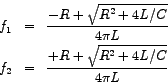
We may solve the last two equations for
and
and therefrom obtain and .
The bandwidth () is therefore given by
.The Quality (Q) factor of the circuit is defined as the ratio of the (current) resonant frequency to the bandwidth.
The smaller is the value of , greater is the value of  , and sharper is the (current) resonance. is also called the selectivity of the circuit. The higher is the value of , the easier it is to select or accept the resonant frequency from nearby frequencies. It may be worth mentioning that another name of the series resonant circuit is acceptor circuit. , and sharper is the (current) resonance. is also called the selectivity of the circuit. The higher is the value of , the easier it is to select or accept the resonant frequency from nearby frequencies. It may be worth mentioning that another name of the series resonant circuit is acceptor circuit.
Phasors
All a.c voltage and currents can be pictorially represented by rotating vectors called phasors. The amplitude of the a.c. voltage or current equals the length of the phasor while its frequency equals the rate of rotation of the phasor in a counter-clockwise sense from a fixed reference direction which is conventionally taken as the x-axis.
How do we represent a phasor mathematically?
The complex notation of an a.c. quantity facilitates expressing a phasor mathematically. To see how, lets take the example of the a.c. voltage across which in complex form reads
 . The amplitude . The amplitude  and the initial phase are the only quantities of importance since the angular frequency of the source, and the initial phase are the only quantities of importance since the angular frequency of the source,  , always remains constant. Hence, we may separate out as follows: , always remains constant. Hence, we may separate out as follows:
 is the exponential form of the phasor corresponding to the complex time-dependent voltage across . It can also be expressed in the rectangular form, viz., is the exponential form of the phasor corresponding to the complex time-dependent voltage across . It can also be expressed in the rectangular form, viz.,
 or in polar form, viz., or in polar form, viz.,
 . Pictorially, the phasor is denoted at time . Pictorially, the phasor is denoted at time  by an arrow of length proportional to making an angle with the horizontal reference line. As t increases, the phasor rotates in a counter-clockwise sense with the frequency . The projection of the arrow onto the vertical `y' axis as it rotates in time gives us the instanteneous sinusoidal variation of the voltage, which turns out to be by an arrow of length proportional to making an angle with the horizontal reference line. As t increases, the phasor rotates in a counter-clockwise sense with the frequency . The projection of the arrow onto the vertical `y' axis as it rotates in time gives us the instanteneous sinusoidal variation of the voltage, which turns out to be
 . .
Calculation of power in a series LCR circuit.
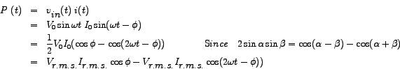
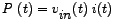
The instanteneous power  delivered to the impedance is given by delivered to the impedance is given by
comprises of a cosinusoidal component
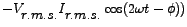 oscillating symmetrically about a constant value oscillating symmetrically about a constant value
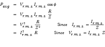
 . This constant value is therefore called the . This constant value is therefore called the Average power. Let us denote it by
 . It may be noted that this value for the average-power could also have been arrived at by integrating over a time-period and then dividing by the value of the time-period. . It may be noted that this value for the average-power could also have been arrived at by integrating over a time-period and then dividing by the value of the time-period.
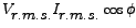
We may express  in terms of the resistance,, and the magnitude of the impedance,, as has been shown before, to be able to write in terms of the resistance,, and the magnitude of the impedance,, as has been shown before, to be able to write
is maximum when equals  . This happens when . This happens when  , the circuit being effectively resistive. On the other hand
acquires the minimum value of zero when equals , the circuit being effectively resistive. On the other hand
acquires the minimum value of zero when equals
 , the circuit being effectively reactive in this case. , the circuit being effectively reactive in this case.
The term, which equals
 is called the power-factor. Since
is always is called the power-factor. Since
is always  and so are and so are
 and and
 , the power-factor varies only between , the power-factor varies only between  and and  . .
One may draw and compare the waveforms for , ,
 and and  .
is observed to vary sinusoidally about
with a frequency, twice that of the frequency of the source, as predicted by theory. We may note that since .
is observed to vary sinusoidally about
with a frequency, twice that of the frequency of the source, as predicted by theory. We may note that since
 and and
 at , so at , so  at , as can be seen from the plots. at , as can be seen from the plots.
It is of interest to gain insight into the physical interpretation of the waveforms. We must remember that we are concerned with the steady state and not the transient state of the circuit. In this steady state, the inductor and capacitor receive energy from the a.c. voltage-source, store it respectively in their magnetic and electric fields during a portion of each half-cycle of the voltage-source, and return all of this energy to the source during the remaining portion of each half-cycle. On the other hand, the energy received by the resistor from the a.c. voltage-source is never returned. The whole of it is dissipated in the resistor as heat or some other form.
The net flow of energy to a passive circuit as the one considered here, in the steady state and in one cycle, is therefore always positive or zero.
As long as the curve is positive, it implies that energy is flowing from the source to the passive elements , and . Whereas, when the curve is negative, it implies that energy is being returned to the source from the passive elements and . A careful look at the waveforms reveal that this occurs during the time the curves for
 and have opposite polarities. and have opposite polarities.
At the (current) resonant-frequency, , the negative portion of the - curve disappears. This signifies that all the energy is dissipated in the resistor and none of it is returned. This is to be expected, since at this frequency, the circuit is essentially resistive, as discussed before.
On the other hand, it may also be observed that if the frequency of the source is made such that the phase-difference between the source-voltage and current waveforms becomes , then the circuit essentially becomes reactive and then the positive and negative excursions of the -curve become equal and
becomes zero.
|
![\begin{eqnarray*}
\mathbf{v_{\big in}} & = & R \; \mathbf{i} + j\omega L \; \mat...
...athbf{i} \; \Big[ R + + j (\omega L - \frac{1}{\omega C}) \Big]
\end{eqnarray*}](LCRresonancetheoryimages/img5.png)