Standing waves and Standing wave patterns in transmission lines
Abhijit Poddar
www.abhipod.com
Standing waves are created by the superposition of incident and reflected travelling waves in an improperly terminated transmission line. By improper termination, what is meant is, the load impedance has a value different from that of the characteristic impedance of the line.
Experience tells us that the teaching and learning of standing waves and standing wave patterns in differently terminated transmission lines can be best accomplished with the aid of animations. Below, I have embedded YouTube videos of animations related to the generation of standing waves and standing wave patterns. The animations have been created by myself, invoking Gnuplot iteratively through a shell script, to read and plot the data generated from simple Fortran programs. Although some Fortran compilers permit invoking of Gnuplot from inside the program itself and the plot of data on the fly, I chose the easier process outlined above.
To learn more about the theory behind standing waves, you need to scroll down this page.
Animation Videos on Standing Waves and Standing Wave Patterns in Transmission Lines
Formation of Standing Wave Patterns in a Lossy Transmission Line
Formation of Standing Wave Patterns in a Lossless Open Circuited Transmission Line
Pure Voltage and Current Standing Wave Patterns in a Lossless Open Circuited Transmission Line
Theory behind Standing Waves and Standing Wave patterns
Signal energy is transmitted through a transmission line from the source or generator to the load or receiver in the form of voltage and current waves. At the load end, part of the signal is reflected back depending on the type of load impedance(![]() ) and the characteristic impedance (
) and the characteristic impedance (![]() ) of the line. The ratio of
) of the line. The ratio of ![]() and
and ![]() determines the reflection coefficient
determines the reflection coefficient ![]() at the load end. The reflection coefficient, defined as the ratio of the reflected voltage to the incident voltage, however, assumes different values as one traverses down the line from the load end towards the source. If
at the load end. The reflection coefficient, defined as the ratio of the reflected voltage to the incident voltage, however, assumes different values as one traverses down the line from the load end towards the source. If ![]() and
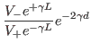
and ![]() be the amplitudes of the incident and reflected voltage waves in a transmission line of length
be the amplitudes of the incident and reflected voltage waves in a transmission line of length ![]() and propagation constant
and propagation constant
![]() (
(![]() being the attenuation constant and
being the attenuation constant and ![]() being the phase constant of the line), then the reflection coefficient
at any point
being the phase constant of the line), then the reflection coefficient
at any point ![]() from the sending end or equivalently at any point
from the sending end or equivalently at any point ![]() from the load end (where
from the load end (where ![]() ) can be expressed through the following equations:
) can be expressed through the following equations:
 |
|||
 |
|||
 |
|||
Again, since the reflection coefficient at the load end can be expressed as:
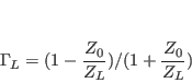 |
The amplitude of the standing wave gives us the voltage standing wave pattern:
 |
If we follow the evolution of the standing wave with time, we will find that its amplitude (![]() ) oscillates between a maximum value (
) oscillates between a maximum value (![]() ) and a minimum value (
) and a minimum value (![]() ), every quarter wavelength apart, the wavelength being that of the voltage wave,
), every quarter wavelength apart, the wavelength being that of the voltage wave,
![]() .
. ![]() is the frequency of the signal being transmitted and
is the frequency of the signal being transmitted and ![]() is the phase velocity of the wave, the value of which is slightly less than the free space velocity (
is the phase velocity of the wave, the value of which is slightly less than the free space velocity (![]() ) of an electromagnetic wave. The distance between two successive maxima or minima turns out to be
) of an electromagnetic wave. The distance between two successive maxima or minima turns out to be ![]() .
Since the position of points corresponding to
.
Since the position of points corresponding to ![]() and
and ![]() remain constant with time, the wave is called a standing wave.
remain constant with time, the wave is called a standing wave.
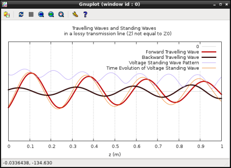
for a lossy line at a particular instant of time.
Figure 1. depicts how a standing wave pattern is generated from incident and reflected waves in a lossy (![]() ) imperfectly terminated (
) imperfectly terminated (![]() ) line. Since the line is lossy,
) line. Since the line is lossy, ![]() and
and ![]() are not constant but a function of
are not constant but a function of ![]() , decreasing progressively with increasing
, decreasing progressively with increasing ![]() . If the line happened to be lossless (
. If the line happened to be lossless (![]() ), then however
), then however ![]() and
and ![]() would have been constant throughout the length of the line.
would have been constant throughout the length of the line.
If a line is terminated in an open circuit (![]() ), a short circuit (
), a short circuit (![]() ) or a pure reactive load like
) or a pure reactive load like ![]() equalling
equalling
![]() , the whole of the incident energy at the load is reflected back (
, the whole of the incident energy at the load is reflected back (
![]() ). The standing wave in all such cases is said to be a pure standing wave. Figure 2. depicts such a pure standing wave for a line terminated in an open circuit (
). The standing wave in all such cases is said to be a pure standing wave. Figure 2. depicts such a pure standing wave for a line terminated in an open circuit (![]() ,
, ![]() ) and assumed lossless.
) and assumed lossless.
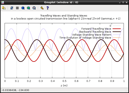
for a lossless open circuited line at a particular instant of time.
For pure standing waves in lossless lines,
![]() and
and ![]() . The points corresponding to
. The points corresponding to ![]() , are now called the nodes and those corresponding to
, are now called the nodes and those corresponding to ![]() are called the antinodes. The instantaneous standing wave, though oscillating with time, is always zero (
are called the antinodes. The instantaneous standing wave, though oscillating with time, is always zero (![]() at the nodes and its magnitude is always a maximum at the antinodes, equalling the amplitude (
at the nodes and its magnitude is always a maximum at the antinodes, equalling the amplitude (![]() ) of oscillation at the particular instant of time.
) of oscillation at the particular instant of time.
Thus we observe, that for standing waves (pure or impure) in any lossless line, ![]() and
and ![]() have the same value throughout the length of the line, and as such, are used to define a parameter called the Voltage Standing Wave Ratio (VSWR) or
have the same value throughout the length of the line, and as such, are used to define a parameter called the Voltage Standing Wave Ratio (VSWR) or ![]() for the line as follows:
for the line as follows:
 |
 |
So far we have been talking about voltage waves and voltage standing wave patterns. We could also obtain current standing waves if we superpose incident and reflected current waves travelling from the source toward the generator and vice versa respectively as follows:
It is very important to note that the reflected current wave is opposite in phase to the reflected voltage wave. Pure voltage and current standing waves and the corresponding standing wave patterns for a lossless line, terminated with a pure reactance (
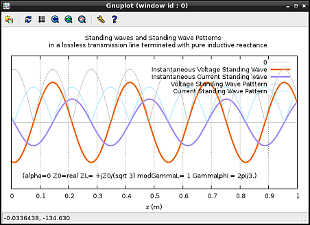
standing wave patterns for a lossless line terminated by a pure reactance
at a particular instant of time.
Interestingly, if the transmission line is perfectly matched (![]() ), there is no reflected wave (
), there is no reflected wave (![]() ). Such a line is called a flat line, since the standing wave patterns turn out to be a straight lines, as shown in Figure 4. VSWR or
). Such a line is called a flat line, since the standing wave patterns turn out to be a straight lines, as shown in Figure 4. VSWR or ![]() for such a line equals 1.
for such a line equals 1.
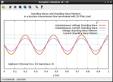
standing wave patterns for a lossless perfectly matched line at a
particular instant of time.
In conclusion, let us ask the question: What is the practical use of the VSWR?
VSWR is used in slotted line measurements of load impedances. A slotted section of a transmission line at the load end is considered for the purpose. A probe is used to sample the electric field and hence the voltage standing wave at different distances from the load and the position of the first voltage minimum (![]() ) in the standing wave pattern is found. The reflection coefficient for a lossless line at a distance
) in the standing wave pattern is found. The reflection coefficient for a lossless line at a distance ![]() from the load end is given by:
from the load end is given by:
| (1) | |||
where
 |
On the other hand, ![]() can be obtained from VSWR measurements, implying we can then obtain
can be obtained from VSWR measurements, implying we can then obtain ![]() which equals
which equals
![]() .
.
Finally, the load impedance can also be expressed in terms of ![]() , as:
, as:
 |
Thus, with the knowledge of standing waves and the VSWR (![]() ), one may obtain the load impedance (
), one may obtain the load impedance (![]() ).
).
© Abhijit Poddar All rights reserved.